Plot eba175 C Allele Proportions¶

Introduction¶

This notebook recreates Supplement Figure 11 from the Pf7 paper - a bar plot which shows the proportions of the eba175 C allele in the major subpopulations.

Eba175 is a vaccine candidate gene with two distinct different allelic forms, known as the F- and C-types. Investigating the prevalence of the eba175 C allele can help assess whether eba175 experiences balancing selection, likely influenced by negative frequency-dependent selection driven by interactions with the human immune system.

This notebook should take approximately two minutes to run.

Setup¶

Install the malariagen Python package:

!pip install -q --no-warn-conflicts malariagen_data
import malariagen_data

     ━━━━━━━━━━━━━━━━━━━━━━━━━━━━━━━━━━━━━━━ 133.2/133.2 kB 2.8 MB/s eta 0:00:00
     ━━━━━━━━━━━━━━━━━━━━━━━━━━━━━━━━━━━━━━━━ 3.1/3.1 MB 42.4 MB/s eta 0:00:00
     ━━━━━━━━━━━━━━━━━━━━━━━━━━━━━━━━━━━━━━━━ 10.4/10.4 MB 77.1 MB/s eta 0:00:00
     ━━━━━━━━━━━━━━━━━━━━━━━━━━━━━━━━━━━━━━━━ 3.6/3.6 MB 57.4 MB/s eta 0:00:00
     ━━━━━━━━━━━━━━━━━━━━━━━━━━━━━━━━━━━━━━ 302.5/302.5 kB 15.8 MB/s eta 0:00:00
     ━━━━━━━━━━━━━━━━━━━━━━━━━━━━━━━━━━━━━━ 138.7/138.7 kB 10.8 MB/s eta 0:00:00
     ━━━━━━━━━━━━━━━━━━━━━━━━━━━━━━━━━━━━━━━━ 20.9/20.9 MB 48.5 MB/s eta 0:00:00
     ━━━━━━━━━━━━━━━━━━━━━━━━━━━━━━━━━━━━━━━━ 8.1/8.1 MB 96.2 MB/s eta 0:00:00
     ━━━━━━━━━━━━━━━━━━━━━━━━━━━━━━━━━━━━━━ 206.9/206.9 kB 20.5 MB/s eta 0:00:00
     ━━━━━━━━━━━━━━━━━━━━━━━━━━━━━━━━━━━━━━ 233.6/233.6 kB 22.0 MB/s eta 0:00:00
?25h  Preparing metadata (setup.py) ... ?25l?25hdone
     ━━━━━━━━━━━━━━━━━━━━━━━━━━━━━━━━━━━━━━━━ 6.7/6.7 MB 60.2 MB/s eta 0:00:00
     ━━━━━━━━━━━━━━━━━━━━━━━━━━━━━━━━━━━━━━━━ 1.6/1.6 MB 34.6 MB/s eta 0:00:00
?25h  Building wheel for asciitree (setup.py) ... ?25l?25hdone

Import required python libraries that are installed at colab by default.

import numpy as np
import pandas as pd
import matplotlib.pyplot as plt
import collections
from google.colab import drive

Access Pf7 Data¶

We use the malariagen data package to load sample data and metadata.

release_data = malariagen_data.Pf7()
sample_metadata = release_data.sample_metadata()

For this figure, we also need to load the eba175 gene allele frequencies in major populations.

This data is available as a .txt file from a web link. We can directly read the data into a dataframe using the read_csv function in pandas!

If you click the left sidebar folder icon, you should see this file appear.

# Read in calls file direct from MalariaGEN website
df_eba = pd.read_csv(
    'https://www.malariagen.net/wp-content/uploads/2023/11/Pf7_eba175_callset.txt'
    , sep='\t'
    , index_col=0
    , low_memory=False
)
# Check shape (should contain 16,203 as this is the number of QC pass samples in Pf7)
print(df_eba.shape)
# View the new dataframe stucture
df_eba.head(3)

(16203, 3)

	f_frac	c_frac	eba175_call
Sample
FP0008-C	0.863946	0.000000	F
FP0009-C	0.003988	0.627346	Mixed
FP0010-CW	0.666667	0.000000	F

Combine data into a single dataframe¶

In order to create the figure, it’s convenient to work with combined data.

We retain all samples from sample_metadata which pass QC (n = 16,203).

# Merge the two dataframes on identical Sample IDs
df_calls = (
    sample_metadata.loc[sample_metadata['QC pass']]
    .merge(df_eba, on='Sample')
)
print(df_calls.shape)
# View the new dataframe stucture
df_calls.head(3)

(16203, 20)

	Sample	Study	Country	Admin level 1	Country latitude	Country longitude	Admin level 1 latitude	Admin level 1 longitude	Year	ENA	All samples same case	Population	% callable	QC pass	Exclusion reason	Sample type	Sample was in Pf6	f_frac	c_frac	eba175_call
0	FP0008-C	1147-PF-MR-CONWAY	Mauritania	Hodh el Gharbi	20.265149	-10.337093	16.565426	-9.832345	2014.0	ERR1081237	FP0008-C	AF-W	82.16	True	Analysis_set	gDNA	True	0.863946	0.000000	F
1	FP0009-C	1147-PF-MR-CONWAY	Mauritania	Hodh el Gharbi	20.265149	-10.337093	16.565426	-9.832345	2014.0	ERR1081238	FP0009-C	AF-W	88.85	True	Analysis_set	gDNA	True	0.003988	0.627346	Mixed
2	FP0010-CW	1147-PF-MR-CONWAY	Mauritania	Hodh el Gharbi	20.265149	-10.337093	16.565426	-9.832345	2014.0	ERR2889621	FP0010-CW	AF-W	86.46	True	Analysis_set	sWGA	False	0.666667	0.000000	F

Distribution of allelic types by population¶

First, we check the frequency of allelic types in the overall dataset before checking in each population.

num_F = np.count_nonzero(df_calls['eba175_call'] == 'F')
num_C = np.count_nonzero(df_calls['eba175_call'] == 'C')
proportion_C = num_C / (num_C + num_F)
print(f"We see {num_F:,} samples with the F allele and {num_C:,} samples with the C allele, \
meaning that overall {proportion_C:.0%} of samples that have an unambiguous call have the rarer C allele.")

We see 7,380 samples with the F allele and 3,364 samples with the C allele, meaning that overall 31% of samples that have an unambiguous call have the rarer C allele.

Now, we will examine individual population allelic frequencies to generate the corresponding figure.

First we define the populations (for more details on populations, please visit the Supplement).

# Define populations in an ordered dictionary
populations = collections.OrderedDict()
populations['SA'] = 'South America'
populations['AF-W'] = 'West Africa'
populations['AF-C'] = 'Central Africa'
populations['AF-NE'] = 'Northeast Africa'
populations['AF-E'] = 'East Africa'
populations['AS-S-E'] = 'Eastern South Asia'
populations['AS-S-FE'] = 'Far-eastern South Asia'
populations['AS-SE-W'] = 'Western Southeast Asia'
populations['AS-SE-E'] = 'Eastern Southeast Asia'
populations['OC-NG'] = 'Oceania'

Next, we need a function to aggregate allele frequencies in each population

# Function to aggregate population frequencies
def my_agg(x):
    names = collections.OrderedDict()
    names['Number F'] = np.count_nonzero(x['eba175_call'] == 'F')
    names['Number C'] = np.count_nonzero(x['eba175_call'] == 'C')
    names['Number F or C'] = names['Number F'] + names['Number C']
    names['Proportion C'] = names['Number C'] / names['Number F or C'] if names['Number F or C'] > 0 else np.nan
    return pd.Series(names)
# Summary table with population aggregates
df_pop_summary = df_calls.groupby('Population').apply(my_agg).loc[populations.keys()]
df_pop_summary

	Number F	Number C	Number F or C	Proportion C
Population
SA	28.0	44.0	72.0	0.611111
AF-W	3111.0	762.0	3873.0	0.196747
AF-C	191.0	30.0	221.0	0.135747
AF-NE	45.0	48.0	93.0	0.516129
AF-E	751.0	210.0	961.0	0.218522
AS-S-E	90.0	15.0	105.0	0.142857
AS-S-FE	712.0	343.0	1055.0	0.325118
AS-SE-W	702.0	741.0	1443.0	0.513514
AS-SE-E	1655.0	1056.0	2711.0	0.389524
OC-NG	95.0	115.0	210.0	0.547619

Make the figure¶

First, we set-up population-specific colour-codes.

# Create an ordered dictionary which maps the codes for major sub-populations -from west to east- to a colour code.
population_colours = collections.OrderedDict()
population_colours['SA']       = "#4daf4a"
population_colours['AF-W']     = "#e31a1c"
population_colours['AF-C']     = "#fd8d3c"
population_colours['AF-NE']    = "#bb8129"
population_colours['AF-E']     = "#fecc5c"
population_colours['AS-S-E']  = "#dfc0eb"
population_colours['AS-S-FE']  = "#984ea3"
population_colours['AS-SE-W'] = "#9ecae1"
population_colours['AS-SE-E'] = "#3182bd"
population_colours['OC-NG']    = "#f781bf"

We are ready to make the bar plot using df_pop_summary data.

# Set the figure size
fig, ax = plt.subplots(1, 1, figsize=(5, 3))
# Set the chart variables
ax.bar(df_pop_summary.index, df_pop_summary['Proportion C'], color=population_colours.values())
# Set the labels
ax.set_xticklabels(df_pop_summary.index, rotation=90)
ax.set_xlabel('Population')
ax.set_ylabel('Proportion of C allele')
# Hide the right spine (axis line) of the plot
ax.spines['right'].set_visible(False)
# Hide the top spine (axis line) of the plot
ax.spines['top'].set_visible(False)
# Set the y-axis limits
ax.set_ylim(0, 1)
# Add a horizontal line showing %50 proportion
ax.axhline(0.5, color='lightgray')
# Adjust figure to ensure everything fits nicely
fig.tight_layout()

<ipython-input-10-1f8c815b50e5>:6: UserWarning: FixedFormatter should only be used together with FixedLocator
  ax.set_xticklabels(df_pop_summary.index, rotation=90)

../../_images/proportion-eba175_29_1.png

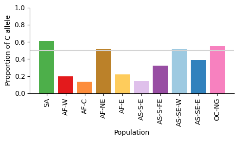
Figure legend: Proportion of C allele of eba175 in different major subpopulations. Horizontal line shows 50% proportion.

Save the figure¶

We can output this to a location in Google Drive

First we need to connect Google Drive by running the following:

# You will need to authorise Google Colab access to Google Drive
drive.mount('/content/drive')

Mounted at /content/drive

# This will send the file to your Google Drive, where you can download it from if needed
# Change the file path if you wish to send the file to a specific location
# Change the file name if you wish to call it something else

fig.savefig('/content/drive/My Drive/Proportion_of_C_allele_by_population_20210720.pdf')
fig.savefig('/content/drive/My Drive/Proportion_of_C_allele_by_population_20210720.png', dpi=480) # increase the dpi for higher resolution

Distribution of allelic types at a more granular level¶

Here we look at the population characteristics organized by country, first-level administrative division, and year.

Then, we identify key summary statistics, minimum and maximum proportions of C allele, within each year and country.

This table was not included in the Pf7 manuscript.

# Group the df_calls by variables (Population, Country, Admin level 1, and Year)
# and apply the custom aggregation function 'my_agg' to calculate the allele frequencies
df_admin1_year_summary = df_calls.groupby(['Population', 'Country', 'Admin level 1', 'Year']).apply(my_agg)
# Print the shape of the resulting DataFrame
print(df_admin1_year_summary.shape)
# Calculate and print the maximum and minimum proportions of the C-type allele
# considering n = number of samples with an F or C type allele called
# min and max C allele proportions where n >= 30
print(f"Max proporiton C (n > 30) = {df_admin1_year_summary.loc[df_admin1_year_summary['Number F or C'] > 30, 'Proportion C'].max()}")
print(f"Min proporiton C (n > 30) = {df_admin1_year_summary.loc[df_admin1_year_summary['Number F or C'] > 30, 'Proportion C'].min()}")
# display 200 rows of resulting df where n > 30
pd.options.display.max_rows = 200
df_admin1_year_summary.loc[df_admin1_year_summary['Number F or C'] > 30]

(297, 4)
Max proporiton C (n > 30) = 0.8048780487804879
Min proporiton C (n > 30) = 0.018518518518518517

				Number F	Number C	Number F or C	Proportion C
Population	Country	Admin level 1	Year
AF-C	Democratic Republic of the Congo	Kinshasa	2012.0	84.0	16.0	100.0	0.160000
			2013.0	51.0	13.0	64.0	0.203125
			2014.0	31.0	1.0	32.0	0.031250
AF-E	Kenya	Kilifi	1996.0	31.0	9.0	40.0	0.225000
			2007.0	42.0	8.0	50.0	0.160000
			2009.0	34.0	5.0	39.0	0.128205
			2010.0	47.0	19.0	66.0	0.287879
			2011.0	39.0	8.0	47.0	0.170213
			2012.0	49.0	16.0	65.0	0.246154
	Malawi	Chikwawa	2011.0	109.0	23.0	132.0	0.174242
	Tanzania	Kigoma	2014.0	54.0	28.0	82.0	0.341463
		Lindi	2013.0	30.0	4.0	34.0	0.117647
		Tanga	2013.0	75.0	15.0	90.0	0.166667
		Tanga	2014.0	70.0	27.0	97.0	0.278351
AF-NE	Sudan	Khartoum	2017.0	17.0	26.0	43.0	0.604651
AF-W	Benin	Littoral	2016.0	53.0	1.0	54.0	0.018519
	Burkina Faso	Haut-Bassins	2008.0	36.0	2.0	38.0	0.052632
	Cameroon	Sud-Ouest	2013.0	95.0	26.0	121.0	0.214876
	Côte d'Ivoire	Abidjan	2013.0	38.0	2.0	40.0	0.050000
	Gabon	Wouleu-Ntem	2014.0	31.0	8.0	39.0	0.205128
	Gambia	North Bank	1984.0	53.0	11.0	64.0	0.171875
		Upper River	2013.0	25.0	14.0	39.0	0.358974
			2014.0	106.0	62.0	168.0	0.369048
			2015.0	33.0	8.0	41.0	0.195122
			2016.0	37.0	13.0	50.0	0.260000
			2017.0	36.0	8.0	44.0	0.181818
		Western	2008.0	43.0	19.0	62.0	0.306452
		Western	2015.0	54.0	26.0	80.0	0.325000
	Ghana	Ashanti	2014.0	87.0	18.0	105.0	0.171429
		Ashanti	2015.0	61.0	13.0	74.0	0.175676
		Central	2014.0	51.0	12.0	63.0	0.190476
		Greater Accra	2018.0	64.0	32.0	96.0	0.333333
		Upper East	2009.0	51.0	8.0	59.0	0.135593
			2010.0	94.0	5.0	99.0	0.050505
			2011.0	45.0	3.0	48.0	0.062500
			2013.0	111.0	8.0	119.0	0.067227
			2014.0	22.0	12.0	34.0	0.352941
			2015.0	121.0	33.0	154.0	0.214286
			2016.0	110.0	44.0	154.0	0.285714
			2017.0	319.0	64.0	383.0	0.167102
			2018.0	356.0	73.0	429.0	0.170163
	Guinea	Nzerekore	2011.0	44.0	11.0	55.0	0.200000
	Mali	Bamako	2013.0	80.0	13.0	93.0	0.139785
		Kayes	2015.0	35.0	15.0	50.0	0.300000
		Kayes	2016.0	27.0	12.0	39.0	0.307692
		Koulikoro	2013.0	49.0	11.0	60.0	0.183333
			2014.0	40.0	1.0	41.0	0.024390
			2016.0	139.0	37.0	176.0	0.210227
	Nigeria	Lagos	2017.0	24.0	14.0	38.0	0.368421
	Senegal	Dakar	2013.0	31.0	13.0	44.0	0.295455
	Senegal	Sedhiou	2015.0	43.0	7.0	50.0	0.140000
AS-S-E	India	Odisha	2017.0	28.0	6.0	34.0	0.176471
AS-S-E	India	West Bengal	2017.0	40.0	5.0	45.0	0.111111
AS-S-FE	Bangladesh	Chittagong	2012.0	23.0	8.0	31.0	0.258065
			2015.0	234.0	132.0	366.0	0.360656
			2016.0	408.0	194.0	602.0	0.322259
AS-SE-E	Cambodia	Pailin	2011.0	26.0	12.0	38.0	0.315789
		Preah Vihear	2011.0	49.0	10.0	59.0	0.169492
		Preah Vihear	2012.0	24.0	8.0	32.0	0.250000
		Pursat	2010.0	34.0	49.0	83.0	0.590361
			2011.0	30.0	47.0	77.0	0.610390
			2013.0	8.0	27.0	35.0	0.771429
		Ratanakiri	2010.0	23.0	9.0	32.0	0.281250
			2011.0	38.0	20.0	58.0	0.344828
			2016.0	17.0	37.0	54.0	0.685185
	Laos	Attapeu	2011.0	23.0	13.0	36.0	0.361111
			2017.0	39.0	19.0	58.0	0.327586
			2018.0	25.0	20.0	45.0	0.444444
		Champasak	2017.0	66.0	15.0	81.0	0.185185
		Champasak	2018.0	54.0	44.0	98.0	0.448980
		Salavan	2017.0	71.0	25.0	96.0	0.260417
		Salavan	2018.0	36.0	4.0	40.0	0.100000
		Savannakhet	2017.0	153.0	66.0	219.0	0.301370
		Savannakhet	2018.0	59.0	54.0	113.0	0.477876
	Vietnam	Binh Phuoc	2010.0	33.0	23.0	56.0	0.410714
			2011.0	53.0	21.0	74.0	0.283784
			2015.0	24.0	8.0	32.0	0.250000
			2017.0	21.0	19.0	40.0	0.475000
			2018.0	85.0	83.0	168.0	0.494048
		Dak Lak	2017.0	46.0	41.0	87.0	0.471264
		Dak Nong	2017.0	18.0	23.0	41.0	0.560976
		Gia Lai	2017.0	104.0	54.0	158.0	0.341772
		Gia Lai	2018.0	75.0	32.0	107.0	0.299065
AS-SE-W	Myanmar	Bago	2012.0	15.0	21.0	36.0	0.583333
		Kayin	2016.0	156.0	182.0	338.0	0.538462
		Kayin	2017.0	117.0	121.0	238.0	0.508403
		Mandalay	2013.0	14.0	32.0	46.0	0.695652
		Tanintharyi	2011.0	8.0	33.0	41.0	0.804878
	Thailand	Tak	2002.0	27.0	13.0	40.0	0.325000
			2003.0	33.0	27.0	60.0	0.450000
			2004.0	31.0	24.0	55.0	0.436364
			2005.0	22.0	15.0	37.0	0.405405
			2008.0	109.0	69.0	178.0	0.387640
			2011.0	18.0	18.0	36.0	0.500000
			2012.0	34.0	32.0	66.0	0.484848
			2013.0	25.0	48.0	73.0	0.657534
OC-NG	Papua New Guinea	East Sepik	2017.0	30.0	24.0	54.0	0.444444

Distribution of allelic types in each country, first-level administrative division and year. This table presents a breakdown of longitudinal and geospatial data concerning the distribution of allelic types (F and C) across 97 combinations of first-level administrative divisions and years for which over 30 samples have either an F or a C type called. The fact that we see both types present in all 97 combinations of admin division and year adds weight to the argument that eba175 is under balancing selection.

MalariaGEN parasite data user guide

Plot eba175 C Allele Proportions

Contents